
“Your model Shaft_Support_1.stl from order #15251 was taken out of production by one of our 3D printing engineers due to design issues: Wall Thickness. See attached image…”
Sound familiar? If you’ve ever had a model rejected by 3D printing engineers because of wall thickness issues, you’re not alone. While this is a very common issue, many 3D modelers may not be aware of how wall thickness is inspected.
Shapeways prints thousands of parts on a daily basis, with a comprehensive system for inspecting wall thickness based on design and materials.
What is wall thickness and why is it so important in 3D printing?
In taking a closer look behind the scenes to understand the calculations, it’s clear that many 3D models look nice on the computer screen but become troublesome during the actual process of 3D printing.
Difficulties arise when models are too thin, and the scenario worsens in the face of less advanced materials and technology. Attempting to 3D print models with thin aspects will likely result in a failed build, along with fragile models breaking in post-processing, in shipping, or in end use.
Although a complete analysis of structural strength would be ideal, that also presents a complex calculational problem, leading 3D printing engineers to employ more simplified empirical measures with wall thickness analysis. If the model has regions which are thinner than some experimental threshold called minimal wall thickness, we assume that the model has high probability to break; therefore, engineers need tools to see where the model is too thin.
Wall thickness visualization in 3D printing requires a straightforward approach
Consider the example of a small vase (shown below as a cross section). The vase has a very small opening, and when we examine it from the outside we have no idea that it has two offending spots with very thin walls.
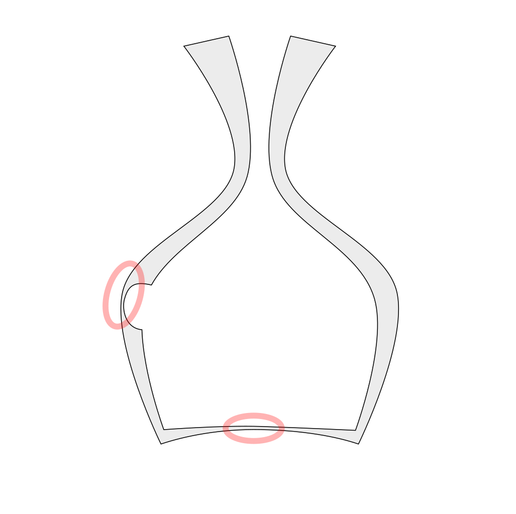
Theoretically speaking, it is relatively easy to find the model thickness at any particular point, by walking inside the model along the internal normal until we hit the opposite surface and exit the model. The distance between entry and exit points is a good approximation to the thickness of the model at that spot.
Manual examination can be extremely time consuming. If you have unlimited patience and time that strategy could work though. All the points on the exterior surface of the vase in the example would eventually be examined and the thin regions would be found and identified. Or would they?
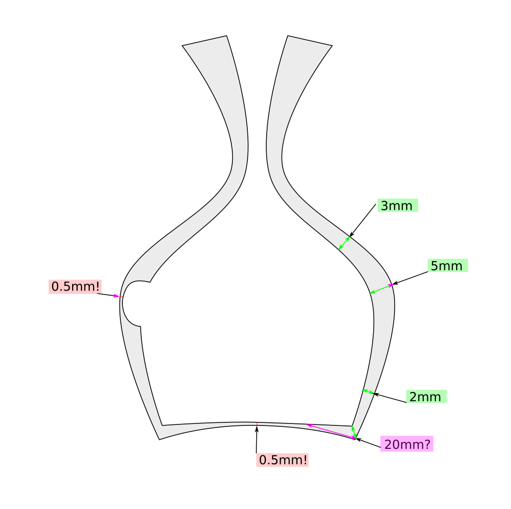
Such approximation to the objects’ thickness may sometimes fail spectacularly. In the example, the 20mm thickness at the bottom right corner of our vase poses a problem. In that spot the internal normal points in the “wrong” direction. There is a much shorter distance to the exit point shown in the green arrow. It is unclear how to select the right direction from the starting point. It looks like we would need to analyze all directions from the starting point and select the direction with the shortest distance. This would be very time consuming.
Rather than this manual approach, a better solution is needed. We developed an algorithm that gives all the tedious work to the computer and provides users with visualization of the problematic regions.
Defining distance function and skeleton calculation in 3D models
First, the definition of wall thickness needs to be defined at a particular point. We start from the definition of signed distance function of an object. Signed distance function (SDF) value at any point in the space is the distance from that point to the closest point at the surface of the object taken with negative sign inside of the object and with positive sign outside of the object. One of the advantages of working with signed distance is the ability to work with both—interior and exterior regions of the object. The SDF value on the surface of the object is zero, and it is approximately linear near the surface.
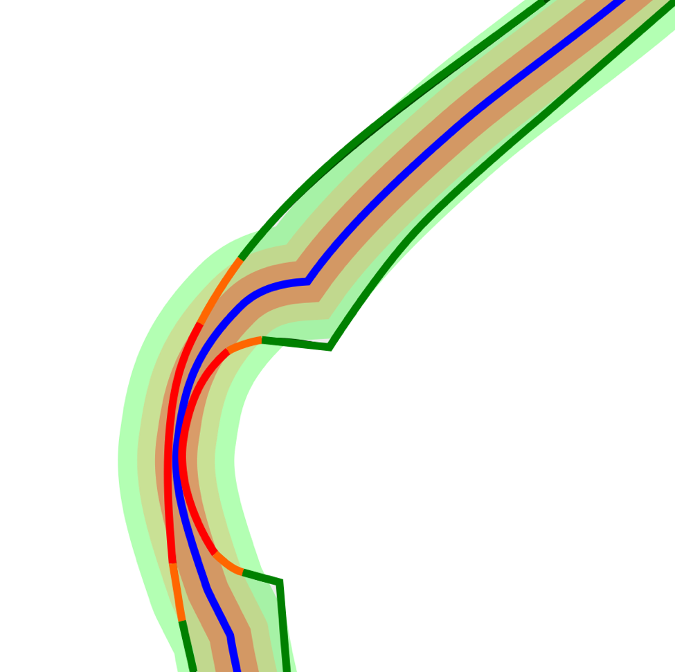
Let’s look at SDF near a region with a thin wall. The SDF is a function of three spatial variables (x,y,z coordinates of a point) and one needs four dimensions to display such a plot. It is simpler and more instructive to look at a plot of SDF along a one-dimensional line (a segment). Only two dimensions are needed to display such a plot, as shown below.
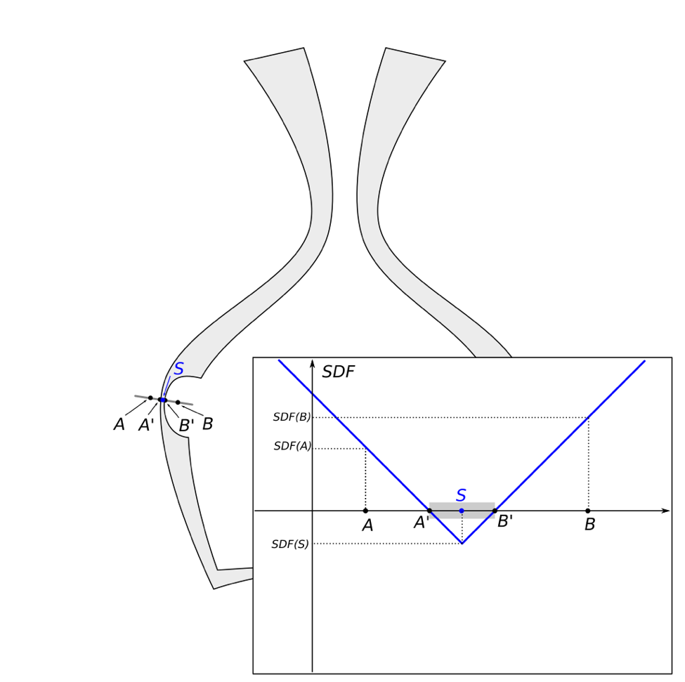
The behavior of SDF along the segment AB is simple to describe. For points inside of the interval AS the closest point on the surface of the object is point A’ and the plot is a simple linear function – the distance to the point A’ with corresponding sign. For points inside of the interval SB the closest point on the object surface is B’ and the plot is another linear function. The special point S is the point in the interior of the object which has equal distances to opposite surfaces of the object (points A’ and B’). The set of such interior points which have equal distance to more than one point on the object surface is called objects’ skeleton. The plot of SDF near skeleton points has a sharp minimum and switches from one linear branch to another linear branch. It is clear that SDF(S) – the value of signed distance function at the skeleton point S is half of the distance between A’ and B’ which is the natural definition of thickness of the objects at that spot. So, we can define the thickness of object as twice of the absolute value of object’s signed distance function at the object skeleton: Thickness = 2|SDF(S)|.[3]
Below is a drawing of the skeleton points in color.
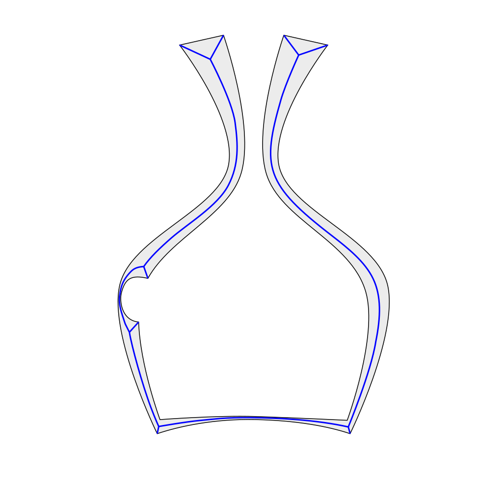
Surprisingly, this skeleton has a lot of unexpected small branches (shown in magenta). Those are the points near the object’s edges. They all satisfy the definition of skeleton (with more than one nearest point on the surface of the object), but they are obviously irrelevant to the object’s thickness. If the initial skeleton were followed, the conclusion would be that all the regions along sharp edges have very small (zero) thickness. This conclusion is clearly unsatisfactory and therefore the skeleton is termed a “dirty” skeleton.
Below are details of the dirty skeleton near the edges.
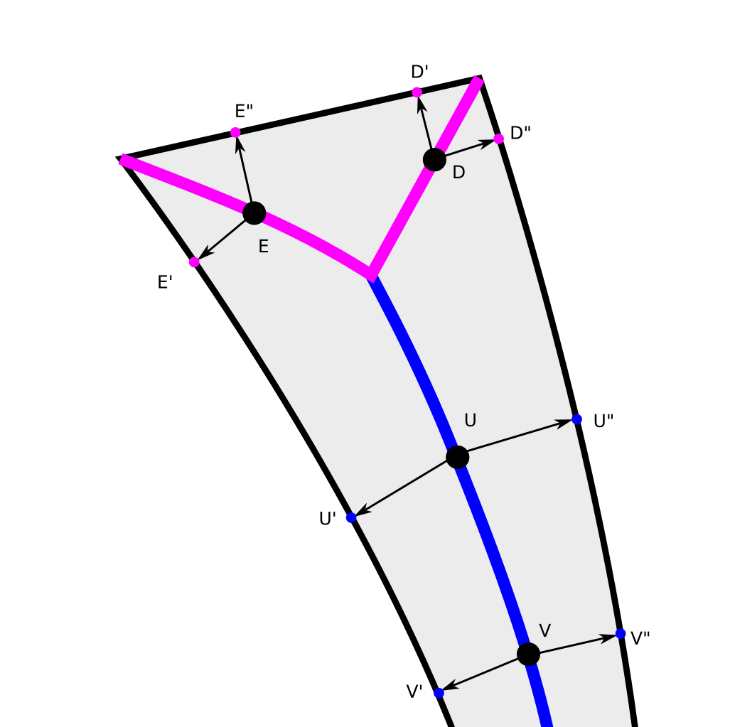
Few skeleton points are marked together with corresponding (closest to them) points on the object’s surface. Points U and V are intuitively good points and are in the middle of the object’s wall. Points E and D are intuitively “bad” points. They correspond to edges and they have to be ignored. The quantitative difference between edge (E and D) and wall (U and V) cases is that those directions to the nearest points are almost opposite in the case of walls, and form an angle close to 90 degrees in the case of edge. This angle can be used as a threshold criterion to remove the edge’s skeleton points and leave only the “clean” skeleton consisting of points corresponding to the object’s walls.
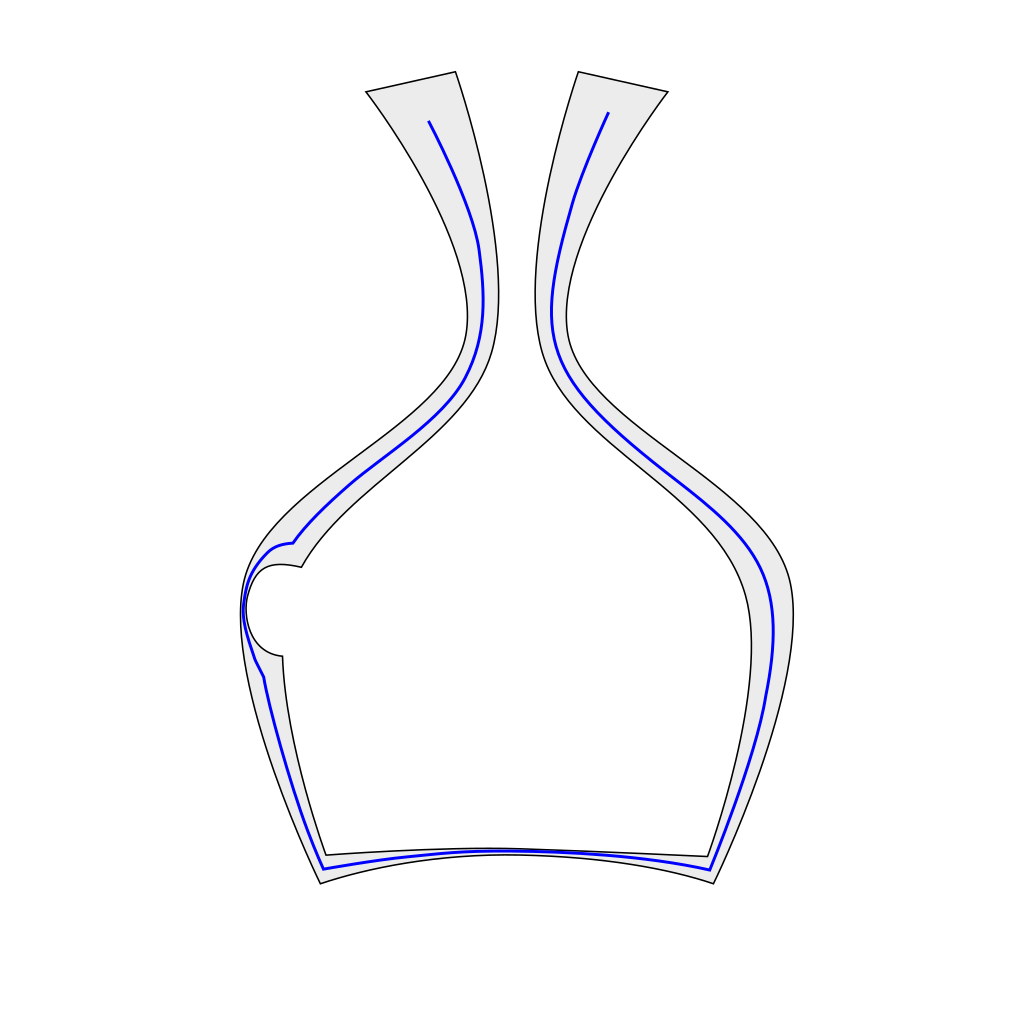
To evaluate more precisely, a “clean” skeleton is needed. Below is an example of the clean skeleton for our example.
Visualizing the skeleton and wall thickness
With the clean skeleton, the calculations of walls and thickness at every point have been determined according to the 2|SDF(S)| formula; however, the skeleton itself may look rather unattractive, and the relation to the original model may not be obvious to the untrained eye. To make the skeleton data accessible, we need to transfer that information to the surface of the original model.
One way to do this is to create a “thick” skeleton, visualizing all the regions with wall thickness below given wall thickness W. Build a shell around the clean skeleton with uniform thickness W – the thick skeleton, knowing that the thickness of the shell is minimal thickness W—everywhere the shell is thicker than the model we can easily see a printability problem. Below any wall thickness thinner than W poses a problem which we highlighted by painting the surface of those spots in red.
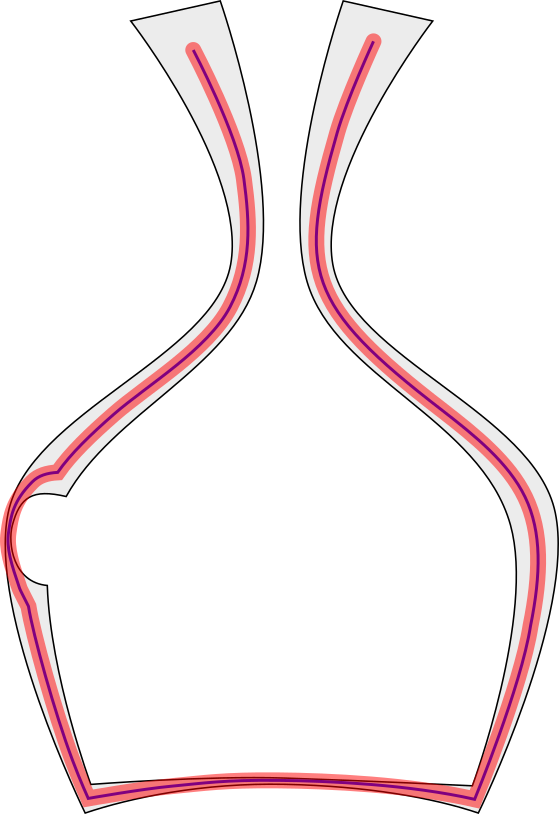
The skeleton can be used in an even more powerful way, employing the distance function to skeleton, mapping distance to skeleton value to color range—using red as an example for distances below minimal thickness, orange for distances slightly larger (say 1.2x minimal wall thickness), and green for everything above 1.5x minimal wall thickness. We can paint the surface of the original model with values of skeleton distance in those colors.
The visualization of thickness of the original model is complete, but simultaneously exact value of model thickness at a specific spot arises from this simple formula: Thickness = 2*DistanceToSkeleton.
That complete procedure is used to create the visualization of the model wall thickness in 3D Tools. It is available only if the algorithm has detected wall thickness problems in your model.
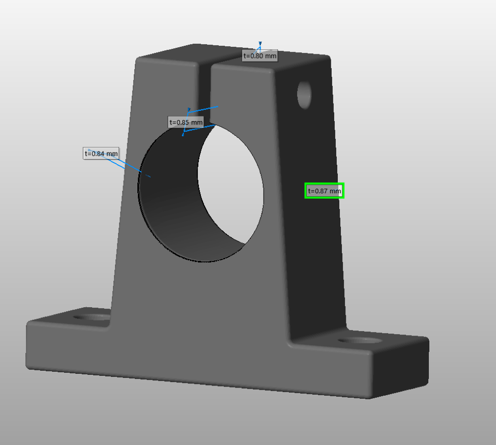
Visualizing in 3D tools
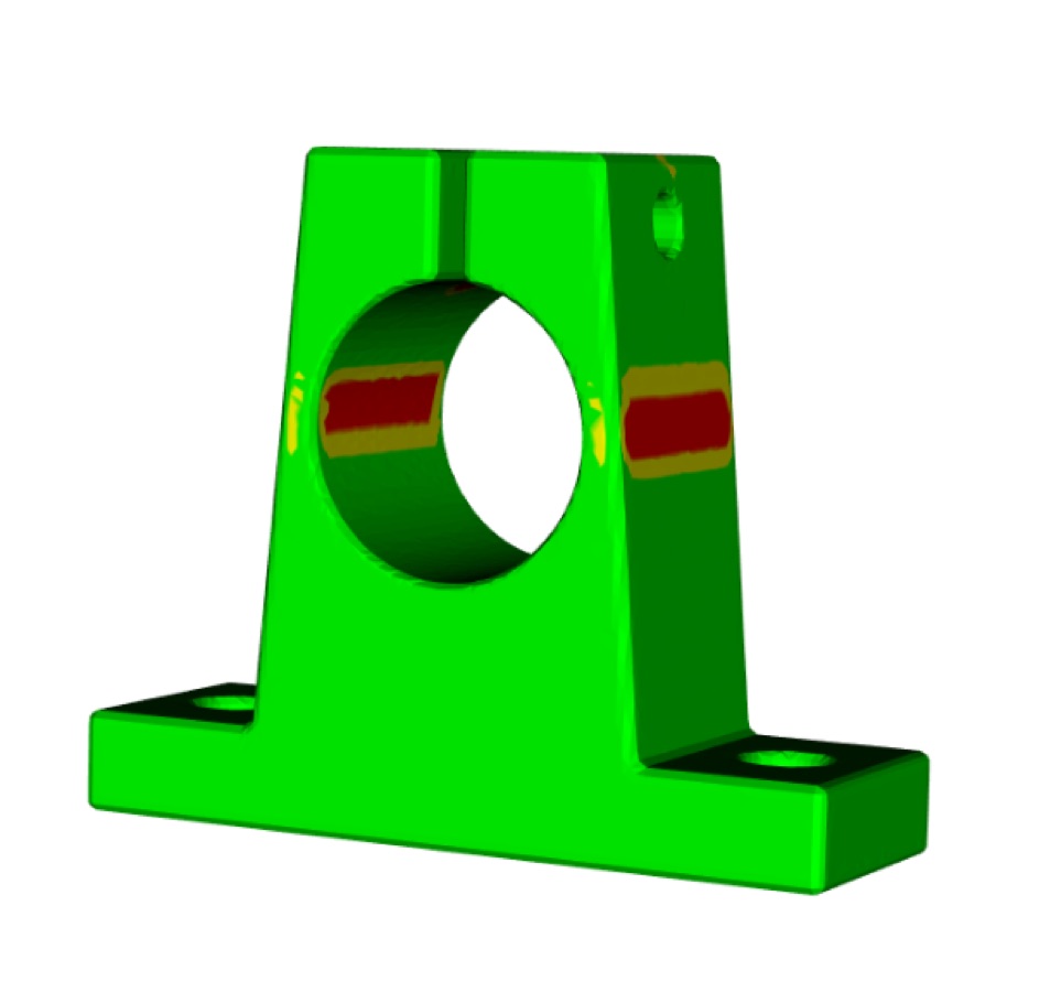
Above is an example of such visualization of a problematic model. This is a small mechanical part, made of stainless steel. That model printed in that material has to have a minimal wall thickness of at least 1mm, but there are few spots where the thickness is only 0.8mm. Those spots are colored mostly in red with some yellow stripes along the boundaries. Those thin spots are in the load-bearing locations of the part and are most definitely the weak spots of the model, requiring the model modification. There are few other places where the algorithm detected the thin walls and highlighted them as well.
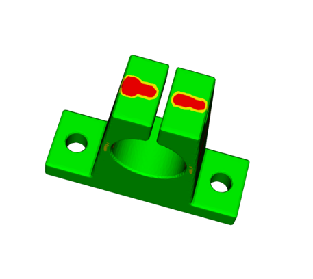
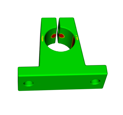
Red spots on these two views above are along the holes going under the surface parallel to the part’s top. Those places are not load-bearing and probably may be ignored, but this decision has yet to be made by a human.
Using what you have learned in this blog, you would probably realize immediately that this model has a printability issue. With the visualization, it is easier to analyze and resolve the wall thickness problem before placing an order. The ultimate goal is success in 3D printing, but if you are still having problems with getting the file to a printable state, 3D printing experts at Shapeways are available to help with questions.
Vladimir Bulatov is a 3D graphics researcher at Shapeways, where he has been focusing on 3D printing algorithms since 2012. Beside computer graphics and 3D modeling, his interests include physics, mathematics, and visual arts.